How to Implement the SWAT MAPS Yield Potential Program to Maximize Your Potential and Cut Costs

Hana Ruf
Regional Manager, East Central SK
hana@swatmaps.com

SWAT MAPS variable rate technology is the first step in maximizing efficiency and productivity through fertilizer, seed, and soil amendments. Once a farm has been fully mapped and the client and their agronomist feel they have a solid fertility plan, they might be wondering what else they can do to improve their practices. The Yield Potential Program (YPP) is for SWAT MAPS clients who want to take their VR potential to the next level. Included in the YPP are unlimited in-season prescriptions, yield analysis, and SWAT CAM.

Unlimited In-Season Prescriptions

Unlimited in-season prescriptions can be made using the SWAT MAP itself, SWAT CAM maps, or NDVI satellite imagery. There are many uses for in-season prescriptions such as on/off or VR fungicides, herbicides, insecticides, plant growth regulators, top dressing, and desiccation/pre-harvest.

Figure 1 is an example of an on/off fungicide prescription that was applied by a ground sprayer using an NDVI map. In this case, areas of the field had minimal crop growth due to dry conditions and sandy soil, and in other areas due to high salinity. The fungicide was turned off in these areas (zones 8-10 on the NDVI map), saving the client $538 on this 150 acre field. If these in-season prescriptions were used across 5,000 acres and fungicide was turned off 20% of the time, in places where it is not needed, the savings alone would pay for the cost of the YPP subscription ($2/ac).

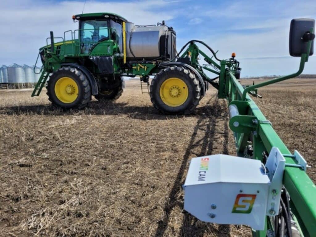
Figure 1. In-season prescription for on/off fungicide for a 150 acre canola field. Prescription is on the left, and resulting application map is on the right.

SWAT CAM

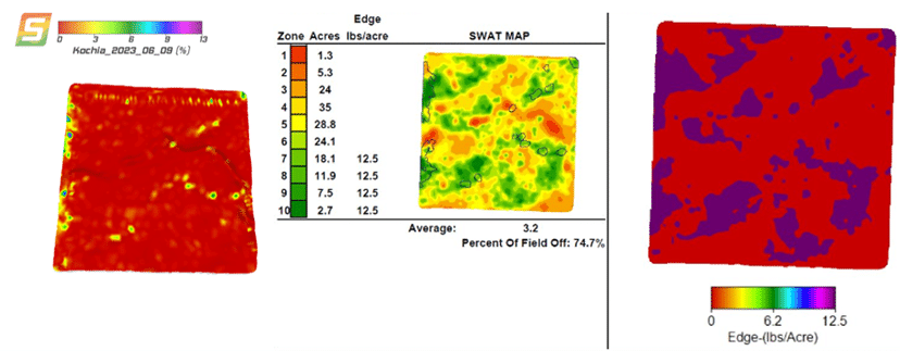
SWAT CAM maps are most often used for top-dressing and herbicide applications. One example of an easy way to save money using SWAT CAM is to target kochia with products such as Authority® (sulfentrazone) or Edge® (ethalfluralin). Figure 2 demonstrates a prescription that was used for an on/off Edge application based on both the SWAT MAP and the kochia map. The Edge is turned on in zones 7-10 on the SWAT MAP, as well as in any places where the SWAT CAM identified kochia plants to ensure good coverage. The Edge was turned off for 74.7% of this 160 acre field, saving $3935.

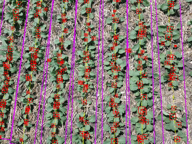
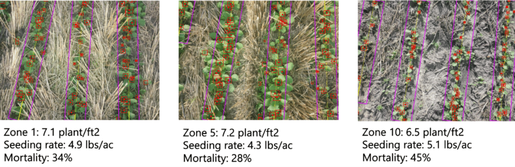
The SWAT CAM is also very useful for helping identify issues in a field such as nutrient deficiencies or drill issues. It is a useful tool for directing scouting efforts and checking on “problem” areas of a field. A quick reference to a SWAT CAM photo in a saline zone 10 can indicate how well the crop is growing there, and if you should adjust your seed or fertilizer rates there in future. The SWAT CAM provides clients and agronomists with unbiased, high resolution plant stand counts for canola, corn, soybeans, and potatoes. Future adjustments to seed rates can be made based on these plant stand counts.

Yield Data

As agronomists, we consider many factors when deciding what fertilizer rates to apply in each zone on a field. We use the SWAT MAP, soil tests, and general knowledge about the field and region to ensure we are not over or under applying seed or fertilizer. As a result, we see many benefits such as increased fertilizer efficiency, reduced lodging, more evenly maturing fields, and increased profitability. However, we are missing an important piece of the puzzle by not knowing exactly how our decisions within a field are affecting yield and ROI. At the end of the season, we don’t get a “report card” to know where the highs and lows were in a field or on a farm. In the YPP, client yield data is cleaned, analyzed, and used to fine tune our decisions going forward.

YPP provides useful data for each field such as actual yield by zone, yield vs. farm average by zone, multi-year yield % of average by zone, stability maps, and profitability maps and graphs. We have been successfully using these tools to identify where we are both overestimating and underestimating yield potential, whether on a zone scale or entire field scale.

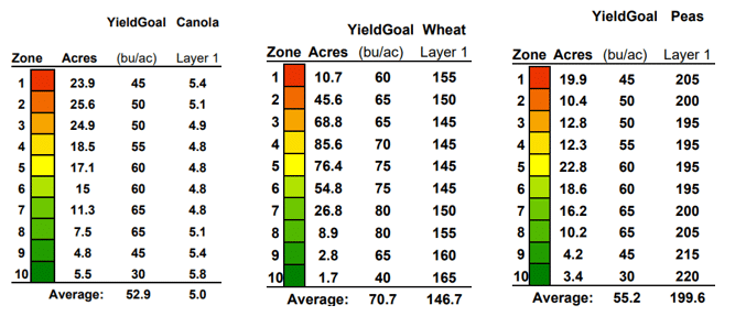
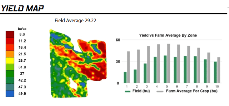
Figure 3 shows a field where we were continuously underestimating the yield potential of the entire field, especially in zones 1, 2, and 10. This was a common trend on this entire farm, so in 2024 we adjusted the yield goals (Table 1.) and fertilizer rates to try and achieve even greater yield in these areas. After a few years of doing this, we can gain confidence in just how much we can push these yields and know what our potential really is. This will allow us to maximize ROI by aiming for our maximum yield potential without overapplying fertilizer to achieve it.

Figure 3. Yield % of Average by zone; 2022 canola actual yields versus target yields by zone.

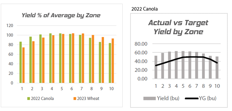
Table 1. Canola yield goal, actual yield, and adjusted yield goal for example field.

Zone	Acres	Yield goal 2022	Actual Yield 2022	Yield Goal 2024
1	6.9	30	53	55
2	41.8	35	60	60
3	85.3	40	62	60
4	95.3	45	63	65
5	106.7	50	63	65
6	122.3	50	62	65
7	156.9	50	61	60
8	99.4	50	58	60
9	26.6	45	52	55
10	8.6	35	51	50

We might also identify fields or zones in which we are overestimating the yield potential. The field in Figure 4 is a poor yielding field historically and has a very sandy zone 1 and 2. When we looked at the actual vs. target yield for each year, we were always well below our target in these zones and on the field average. We knew the yield was poor in zones 1 and 2 and did adjust the yield goals and fertility for that, but we were still overestimating the yield potential even in years with adequate rainfall. Looking at the yield vs. farm average by zone and seeing how poor this field performs compared to the rest of the farm, we decided since this is a higher risk field we might be better off scaling back the fertilizer and yield goals and allocating that budget to better performing areas on the farm. This will help mitigate the risk and manage inputs properly.

Figure 4. A poor performing field with very sandy zones 1 and 2 that consistently yield lower than the farm average.

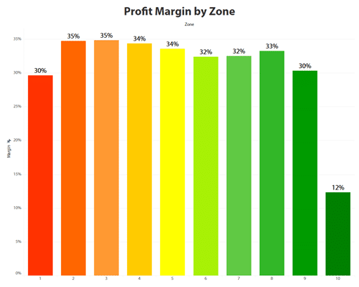
Clients can provide their input costs and selling prices to attain profitability maps and analysis through the YPP. This can help us improve margins and increase profitability both in good producing zones and troublesome zones. Zones 6 and 7 in the field in Figure 5 are at 32% of the profit margin (profit margin = profit/income). The yield data analysis provides this information, and then the client and agronomist can determine the “why.” We might be able to use SWAT CAM images to provide us with more information. We can then decide if there is a way to increase these margins. Is the solution in the seed or fertilizer rates? Do we need better drainage? If the profit margin in zones 6 and 7 can be increased by 2%, that would be an additional $30/ac. At 160 acres, that is $4800.

Figure 5. Profit Margin Analysis by Zone for a 160 acre field.

Summary

There are many use cases for the Yield Potential Program. Unlimited in-season prescriptions provide clients with an efficient and cost reducing alternative for applying pesticides. SWAT CAM provides options for directing scouting efforts, diagnosing and assessing issues in a field, and unbiased plant stand counts. The yield analysis component has many benefits which all help to fine-tune seed and fertilizer management and improve profitability.

For more information or to sign up for the Yield Potential Program, call 1-800-421-4099 today!

High resolution plant stand assessments with SWAT CAM

Brandon Smith
Regional Manager, Central SK
brandon@swatmaps.com

Having a consistent and even plant stand across a field is beneficial in achieving even maturity and maximizing yield. Consistent maturity is critical for fungicide staging (especially for fusarium head blight in wheat) as well as harvest timing. At Croptimistic we use SWAT MAPS to not only vary rates of fertilizer but also to vary seeding rates. This allows us to have a nice, even plant stand. Conditions in the defined SWAT zones will affect seedling mortalities, therefore we can increase seeding rates in those zones to even out plant stands (Figure 1). Typically, zones 1-2 and zones 9-10 will have the highest mortality depending on the field’s soil properties and moisture conditions. These zones will have the highest seeding rates. Zones 1-2 are drier areas of the field that are water-shedding and can often have lighter textured soil, tend to have shallower seeding, and can dry out when it is hot and windy, which increases mortality. Zones 8-10 can often be “mudded in” as these areas are wet when seeding, can have permanent soil issues such as salinity, peat, or sodicity, and these factors again, will increase seed mortality. In the end, we typically prescribe the same amount of seed as we would for a flat rate, but redistribute it to optimize the final plant stand.

Figure 1: Example of VR canola, wheat, and pea seed prescriptions from left to right. Increasing the seeding rates in Zones 1-2 and 8-10, as these zones have higher mortality.

It is important that we assess our VR seeding rate strategies to ensure that we are hitting our plant stand targets across SWAT zones. Before SWAT CAM, the process for doing this was by manual plant stand counts, which involved counting a few different areas in each zone to come up with an average plant stand count across zones and across the field. This method was very labor intensive and low resolution, since we are counting limited locations in a few fields across a farm to assess our VR seed strategy. As we know, different fields will have different seeding conditions, soil types, and therefore different mortalities. Manual plant stand counts are not able to capture all variability within every SWAT zone across a farm.

Figure 2: SWAT CAM system mounted to sprayer boom

SWAT CAM is a camera system that is mounted to a sprayer that is automatically capturing 1000s of images on every field, running those images through a machine learning algorithm, and getting plant stand counts for several crops. As of today, SWAT CAM can count individual plants in canola, corn, soybean, dry bean, faba bean, and potato. In 2024 we will be beta testing plant stand counts for cereals and lentils.

Figure 3: Example of SWAT CAM image with canola plant stand count model.

SWAT CAM allows us to accurately assess our VR seed strategies on the crops that we have plant count models for. As shown in Figure 3, we can count individual canola plants and calculate the average plants per square foot in that image; in this example the average was 5.5 plants per square foot. The seeding rate in this zone was 4.3 lbs/ac and calculated mortality was 44%, which is slightly better than the industry standard for canola seed.

Figure 4: Canola plant stand count by zone with calculated mortalities.

With 1000s of counts across the field analyzed by SWAT zone we can then get an average of the whole field and an average plant stand for each SWAT zone. This data can help us to adjust our VR strategies. For example, if SWAT zone 1 has a higher plant stand than we were expecting, and zone 1 received the highest seeding rate, then in the future we can consider decreasing the seeding rate resulting in reduced seed costs. Another example may be that certain fields on the farm tend to have lower mortality across the whole field and the plant stand is always higher on those fields. This is another opportunity to decrease the seeding rate. Alternatively, fields with higher-than-expected mortality should be investigated further. Do seeding rates need to increase or are there other factors causing the high mortality that need to be altered, such as residue management, fertilizer placement and seed-placed rates?

SWAT CAM data allows us to calculate mortalities across SWAT zones by comparing the seed rates applied to the actual plant counts calculated by SWAT CAM. Automation of this process allows us to capture optimized plant stand counts across full farms at a low cost. SWAT CAM increases our confidence in our plant counts such that we can make better decisions and adjustments to variable rate seed strategies.

Using SWAT MAPS to optimize fertility recommendations, reduce crop Inputs, and save $$$

Sean Barath
Precision Agronomist
sean.barath@swatmaps.com

Introduction
Every fertilizer recommendation should start with soil test data. Without soil test data you would basically be making blind recommendations, based on yield goals and crop uptake/removal tables. This is not an ideal method of nutrient planning as you could either over or under apply certain nutrients.

Soil Testing
Composite soil testing (Table 1) can be a good starting point for making fertilizer recommendations for flat rate applications; however, it only captures soil nutrient levels in the mid-slope areas of fields, leaving out important information on soil nutrient levels in depressions or hilltops. Implementing zone-based soil sampling (Table 2) along with the use of SWAT MAPS variable rate seed and fertilizer can help producers get their best ROI on inputs and save money.

Table 1. Example of composite soil sampling test results.

Table 2. Example of zone-based soil sampling test results.

Right away, the zone soil test results in Table 2 show some potential cut back on nitrogen and phosphorus rates in upper and lower SWAT MAPS zones. Zones 1-2 are hilltops where the yield is most limited by low moisture levels, whereas zones 7-10 start getting into yield-limiting levels of salinity. There are already higher soil nitrate and phosphate levels in these areas which will also influence the recommendation for these zones. The zone soil test also sheds some light on other soil factors that the composite sample does not show. The pH levels are elevated in zones 1-2 and 7-10, OM differences between zones are significant and sulfur and zinc levels in zone 1-4 are lower.

Fertility Recommendations

The process of making fertility recommendations based on a SWAT MAP is simply not a button to hit that gives a recommendation. Agronomists are in contact with the farmer early in the fall to discuss any fall fertilizer passes, and then again in the winter for spring plans. In some cases, the grower has a set fertilizer budget to work with, while other growers want a fertility plan more aligned with yield goals and soil test results. Once agronomists have the grower's intended fertility plan, VR recommendations can begin.

Soil test results (Table 2) are the main tool to determine crop demand for a certain yield goal. The soil test is also very useful in determining the soil N supply, including left-over nitrates, organic matter credits, and N credits for cases like previous pulse crops, broken up hay/alfalfa land or previous manure applications. A critical soil test N level of 20 lbs/ac is used. If levels are below this threshold at year end, the crop was potentially starved. If levels are higher than 20 lbs/ac, the crop was supplied with too much N, other factors limited yield and nutrient uptake, or the soil mineralized more nitrate in season that the crop didn't use. When making recommendations, the crop is supplied with enough N for the yield goal while maintaining the 20 lb/ac level at year end. N credits can be tricky as there aren't absolute numbers for the mineralization rate and amount of N coming from the organic matter, pulse crop residue, old hay residue, or manure applications. Organic matter credits can range from 6-8 lbs of N per % OM but can be unpredictable in terms of the above-mentioned practices. When making zone-based recommendations with N credits, the size of credit given can also be based on the landscape position of the field. Zones 1-2 usually have the lowest N credit per % OM as these areas tend to be driest, resulting in less mineralization. In Zones 3-8, credits gradually increase due to higher mineralization potential in lower landscape areas as soil moisture and organic matter content increases. Zones 9-10 can have the highest N credit unless poor health limits microbial activity.

**Figure 1. Nitrogen Recommendation for a 45 bu/ac average canola crop.**

The example SWAT MAPS Field in Figure 1 has soil nitrate levels of 15 lbs to 104 lbs. The zone trend is common, especially after drought years where the zone 1-2's (hills) and zone 7-10's (saline areas) both have high soil nitrate levels where the crop use was low. The organic matter levels range from 4.6 to 6%. The average canola yield goal for this field is 45 bu/ac; however, yield goals per zone do vary based on zone characteristics that limit yield potential. Canola is a heavy user of N, using roughly 3 lbs N per bushel of grain produced. Using the yield goals from Figure 1 would result in crop demand ranging from 105 lbs actual N to 150 lbs actual N. Crop demand is an easy starting point to begin making the recommendation. Total soil supply includes residual nitrates plus N credits from organic matter, minus any losses that may happen and minus the 20 lb/ac year end critical level. Losses are hard to predict but N losses in lower, saturated areas within a field due to denitrification are more likely to happen. There can be leaching losses in sandy areas as well with very wet conditions. Once soil supply is determined, this amount is subtracted from crop demand and the remaining fertilizer requirements are made into a VR report.

In a SWAT MAPS recommendation for P, 15 ppm Olden-P generally is the critical level. Less than 15 ppm is low and zone(s) testing low will receive higher P rates to increase the soil test P level to above 15 ppm. If the soil test level is higher than 15 ppm, maintenance rates are applied to the zone(s) to maintain the soil test levels above 15 ppm. If soil test levels are high, to a point where they become an environmental concern, lower P rates are applied to allow the crop to mine the excess P from the soil. In the SWAT MAPS field example, the soil test in Table 2 shows zones 3-6 are well below the critical level of 15 ppm. These areas are the focus for the VR phosphate application. Zones 1-2 and 7-10 soil test levels are above the critical level and will receive maintenance rates. Depending on yield limiting factors, lower P rates may be applied to allow the crop to mine from the soil. Saline areas and fields that have had excessive manure applications in the past are some examples of where mining soil P instead of maintaining the levels would occur. Table 3 has recommended application rates from AGVISE Laboratories for P based on soil test levels and yield goals. Canola is a heavy user of P, removing roughly 0.9 lbs of P₂O₅ per bushel of canola grown and this needs to be taken into consideration when making P recommendations for canola. The soil test results for the example field in Figure 2 are showing soil P levels down to 8 ppm. According to this recommendation chart and the yield goal, it would need to be 40-45 lbs of actual P₂O₅ just to maintain this soil test level; however, applying higher rates to build the soil P level is a good idea.

Table 3. Phosphorus fertilizer recommendation guide from Agvise Laboratories.

Figure 2 shows an example VR report of the N & P recommendations for the example field. As you can see, the fertility rates do vary significantly depending on zones, soil test data and the overall crop demand.

**Figure 2. Example VR report for SWAT MAPS field.**

Variable rate vs. Flat Rate Applications
You might be wondering how variable rate will give you the best ROI on your inputs and possibly save you some money. The soil test results from Table 1 and Table 2 would result in very different fertilizer applications. A recommendation based on the composite soil test would result in high application rates being applied to the whole field. The zone-based soil test is telling a different story, where there is opportunity to rely on residual N and P levels to supply the crop with part of the fertility demand along with accounting for yield limiting factors like the salinity in Zones 7-10. In Figures 3 and 4, variable rate vs flat rate urea comparison shows how effective SWAT MAPS can be at saving product from over application in areas of the field that don't need the extra fertility.

**Figure 3. Urea VR vs FR comparison for the example field.**

**Figure 4. Phosphorus VR vs. FR comparison for the example field.**

Conclusion
Composite soil testing is a good start when making fertilizer recommendations; however, this sampling method misses important details within areas of a field like nutrient levels, pH differences, salinity, organic matter, etc. Zone-based soil sampling and SWAT MAPS Variable Rate is the most effective way to capture all the variability within a field. In the variable rate vs. flat rate example, the grower would save 37,875 lbs of urea and 19,144 lbs of MAP just by using SWAT MAPS on this field. That is a large amount of product saved and can result in product reallocated to other fields or saved money that can be invested into other areas on the farm. Talk to your SWAT MAPS service provider about how they can help you get the best return on your crop inputs and save money with SWAT MAPS Variable Rate.

Groundtruthing to select the correct SWAT MAP: What about peat?

A SWAT MAP is a map that sets the framework for a field’s soil potential and therefore management plan. This management could be for any or a combination of fertility, seed, or soil applied herbicides. By understanding the potential of soils within a field, we can maximize them, but we need to ensure we have the right map.

The first step is mapping a field with a SWAT BOX to collect electrical conductivity, elevation, and topography data which allows the creation of maps that utilize these layers in different weightings. Depending on the soil type and geographical area, the weightings will differ. This is where the critical step of ground-truthing comes in to determine the correct layers in a SWAT MAP. A trained SWAT agronomist in the field analyzes the data layers to decide what map best represents the field.

Available data layers will also include depressions, hills, and water flow paths. The agronomist uses these layers with background imagery, soil survey information, and possibly yield data if it is available. Then soil cores down to 2 feet are taken in several areas to determine any differences in soil color or horizons. As the agronomist travels the field, stubble differences, weeds, or any regrowth can help indicate how certain areas should be zoned.

Sometimes there are unique soils that are difficult to capture in the typical data layers, and this is where being in the field, looking at the soil and stubble can help identify proper SWAT zones. One example of this is Organic order or peat soils. Because peat presents unique challenges, it needs to be managed on its own and sometimes requires a modification on the SWAT MAP to ensure it is represented well.

Peat soils can mineralize an incredible amount of N, leading to excessive vegetative growth, lodging, and delayed maturity. Here is an example of the total N that was measured in a field with peat soil in zones 9 and 10:

Table 1. Organic matter, total N, and resulting estimated pounds of organic N in 0 to 8”.

Zones	OM (%)	Total N (%)	Total Organic N (lbs, to 8” depth)	1% of Total N (lbs)
1,2	4	0.231	6,160	62
3,4	4.6	0.275	7,333	73
5,6	6.9	0.325	8,667	87
7,8	9.9	0.443	11,813	118
9,10	27.1	0.959	25,573	256

In this example, if only 1% of the total N is mineralized, zone 10 would potentially have 256lbs of N become available!

The mineralization potential is impacted by organic matter as well as moisture (Schoenau, 1995). Peat soil in a field will often correlate with lower landscape position where water tends to collect and have increased mineralization potential due to moisture availability.

Organic matter binds copper more tightly than any other micronutrient (The Fertilizer Institute), so copper deficiencies occur more often here, and the critical levels used are higher than in mineral soils.

Manganese, while not often tested in a routine soil test, is another micronutrient that can be unavailable in peat soils as it becomes oxygenated and is in an unavailable form. Oats are more susceptible to this deficiency, and this has been seen in northern Alberta, where these soils are found fairly frequently.

Table 2. SWAT Zones and correlating organic matter and Mn tissue test results in oats, N Alberta.

Zones	OM	Tissue test Mn
1,2	5.5	109 (high)
5,6	7.1	57 (sufficient)
9,10	64.0	9 (low)

Another characteristic that differs with managing peat is the ideal pH. While in mineral soils we don’t want to see a pH lower than 5.5 , and will adjust with amendments such as lime to target higher than this, in organic soils we don’t want to adjust higher than 5.5 or nutrient availability issues will arise (UMN Extension, 2023).

Here is an example of a field that had an area with peat that needed to be isolated. Prior to mapping, there happened to be oats on this field which are relatively tolerant to low pH. It was also a dry season, so low lying peat depressions were rather dry. This meant stubble was consistent across the field. Driving across the field, the peat was evident, and soil cores revealed areas with different peat profiles. Zones 7-8 had only about 6 inches of peat on top, whereas zone 10 had close to 18 inches of peat. Topography and depression layers also helped to segregate these areas. Background imagery from previously wet years was also helpful to find the edges of impacted areas for zoning.

Figure 1. EC Layer

Figure 2. Original SWAT MAP

Figure 3. Modified SWAT MAP to improve management areas

Figure 4. Soil test results from 0-8" and 8-16", NE Alberta

This example shows the importance of all the steps that go into creating the best possible SWAT MAP, and the map accuracy is confirmed by the soil test results, where there are drastic differences between zones.

Peat can differ in depth, how well it's drained, and its mineralization potential but in all cases, needs to be managed independently.

All the data layers collected while mapping and compiled in SWAT MAP creation are invaluable to the framework of selecting the appropriate SWAT MAP. Being in the field and looking at all variables is a critical step to ensure we have the most detailed map possible to base sound recommendations from.

References

J.J.Schoenau, Department of Soil Science, University of Saskatchewan. Understanding the Role of Mineralization in Supply of Plant Available Nitrogen, 1995.

The Fertilizer Institute. (n.d.). Essential Elements; Copper. https://www.tfi.org/sites/default/files/tfi-copper.pdf

The Fertilizer Institute. (n.d.). Essential Elements; Manganese. https://www.tfi.org/sites/default/files/tfi-manganese.pdf

(n.d.). University of Minnesota; Liming. https://extension.umn.edu/nutrient-management/liming